Every attribute on every shape, what each format actually contains, and the three things that catch people out on import. Measured from the shipped sample archives, not quoted from the specification sheet.
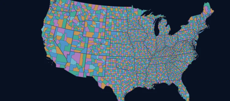
The family is a boundary file and a centroid file. They are not alternatives — most projects want both, and they answer different questions.
| Product | What it contains | Records | Attributes |
|---|---|---|---|
| ZIP Code Boundaries | Only the ZIP Codes that have a defined delivery area, as polygons. This is what you draw a map with. | ~32,000 | 19 |
| ZIP Code Centroids | The universe of ZIP Codes, one point each — both the center of every polygon above and the PO Box and Unique ZIP Codes that have no area at all. This is what you geocode against. | ~41,000 | 18 |
The centroid file is the bigger one, and that is the point. A PO Box ZIP Code has no delivery area — mail goes to a counter in a building — so it can only ever be a point. If you work only from the boundary file, those ZIP Codes do not exist in your data at all, and a customer address in one of them silently fails to match. Centroids carry the full set.
Centroids are placed, not computed. For a polygon ZIP Code the centroid is a modified geographic center, adjusted so it is guaranteed to sit inside its own polygon — a naive center-of-bounding-box lands in the sea for a coastal ZIP and in the neighboring ZIP for a crescent-shaped one. For a point ZIP Code it is placed at the Post Office or the recipient's own address.
Each sample archive also carries ZIP Code Boundaries Product Documentation.pdf
and a copyright notice. The documentation was refreshed in August 2026 — the format list now
matches what ships, and the one remaining difference (the ZIPTYPE
value spellings) is flagged in the dictionary below.
Every attribute attached to every shape. 19 on the Boundary product,
18 on the Centroid product — identical except that Centroids carry no
COLOR. Names are read from the shipped files, not from the
specification sheet.
A ZIP Code is not really a shape. It is a set of addresses on streets, so every polygon in this product is a considered representation of one — built by dissolving USPS carrier route boundaries and extending them so ZIP Codes tile the country. That is why it looks different from the Census ZCTA file, and why the delivery counts below exist at all.
ZIPTYPE does not tell you the geometry type. Most PO Box and
Unique ZIP Codes are points, but not all of them — pooled across our four
samples, 216 PO Box records are points and 26 are polygons; 52 Unique are points and
17 are polygons. Branch on the geometry, never on the type code.
| Attribute | Description | Type | Boundaries | Centroids |
|---|---|---|---|---|
| Identity 5 fields | 5 | 5 | ||
ID | Row identifier within the release. Not a stable key across releases — join on ZIP, not on this.Example: 475 | Integer | ||
ZIP | The 5-digit ZIP Code. Not always numeric: filler records carry a 3-digit prefix followed by MH or MX, e.g. 901MH. Import as text, and keep the leading zero.Example: 02108 | Char(5) | ||
NAME | Primary postal town name for the ZIP Code.Example: BOSTON | VarChar(40) | ||
ZIPTYPE | One of four: NON-UNIQUE ordinary street delivery, PO BOX a Post Office box facility, UNIQUE a single high-volume recipient such as a university or agency, and FILLER an MH/MX area with no mail delivery. This does not tell you the geometry type — see the note above the table.Example: NON-UNIQUEHeads up: The documentation spells these NON_UNIQUE and PO_BOX with underscores. The data ships NON-UNIQUE and PO BOX — hyphen and space. Match on the shipped spelling. | VarChar(20) | ||
RELVER | Release version, as YYYYMM — 202405 in this release. Stamp it on your import so you can tell which vintage a row came from.Example: 202405 | Char(8) | ||
| Where it is 5 fields | 5 | 5 | ||
STATE | State abbreviation. A ZIP Code can cross a state line; the value here is the state used in mailing addresses for that ZIP.Example: MA | Char(2) | ||
STATEFIPS | State FIPS code. Ships with its leading zero — read it as text.Example: 25 | Char(2) | ||
COUNTYFIPS | Full county FIPS code (state + county). Leading zero is significant.Example: 25025 | Char(5) | ||
COUNTYNAME | County name. A ZIP Code can cross a county line; the same mailing-address rule applies as for state.Example: SUFFOLK | VarChar(60) | ||
S3DZIP | The first three digits of the ZIP Code — the sectional center facility. Useful for rolling territories up without a separate join.Example: 021 | Char(3) | ||
| Centroid 3 fields | 3 | 3 | ||
LAT | Latitude of the ZIP Code centroid. For a polygon ZIP this is a modified geographic center, adjusted so it is guaranteed to fall inside the polygon — a naive centroid can land outside a crescent-shaped or multipart ZIP. For a point ZIP it is the Post Office or the recipient's address.Example: 42.358497000000000 | Float | ||
LON | Longitude of that same centroid.Example: -71.063530999999998 | Float | ||
ENCZIP | Enclosing ZIP Code. On centroid records — PO Boxes and Unique facilities, which have no delivery area of their own — this is the ZIP Code whose polygon physically contains that point, so you can tell which delivery area they sit in. The column ships in the Boundary file too, but is always blank there.Example: 19104Populated on 33% of records in our samples. | Char(5) | — | |
| Delivery counts — the part ZCTA cannot give you 5 fields | 5 | 5 | ||
TOTRESCNT | Total residential deliveries in the ZIP Code. This and the four counts below are actual delivery-point counts, which is what separates this product from a census-derived approximation.Example: 2190 | Integer | ||
MFDU | Multi-family deliveries — broadly, apartments.Example: 1766 | Integer | ||
SFDU | Single-family deliveries — broadly, houses.Example: 424 | Integer | ||
BOXCNT | Residential PO Box deliveries.Example: 0 | Integer | ||
BIZCNT | Business deliveries. Includes business PO Boxes.Example: 1159 | Integer | ||
| Cartography 1 field Boundaries only | 1 | 0 | ||
COLOR | A four-color map index: a small integer chosen so that no two adjacent ZIP Codes share a value. Shade your polygons by this and neighbors never collide, without you computing an adjacency graph. Boundaries only — the Centroid product has no COLOR.Example: 4 | Integer | — | |
Attribute names, fill rates and examples measured from the May 2024 sample archives (841 records across four extracts); descriptions from the product documentation included with every download. Datum is WGS84 / EPSG:4326 in every format.
All eight ship in every download at no extra cost, so this is not a purchase decision — but it is a real technical one, because they do not all carry the same records.
A shapefile holds exactly one geometry type. These exports are declared
Polygon, so the point-only ZIP Codes — PO Box and Unique — are
written into the shapefile with empty geometry: the attribute row is there, the shape
is not. They will not draw, will not match ST_Contains, and
ST_Area returns zero, with no error anywhere. Measured across our four sample
extracts that is 3 of 45 records in the small sampler and 196 of 498 in LA
Metro — the denser the metro, the more PO Box ZIP Codes, the bigger the hole.
If you need every ZIP Code, use GeoJSON, WKT, CSV or one of the SQL formats.
| Format | Carries point ZIPs | Carries attributes | Best for |
|---|---|---|---|
| GeoJSON.geojson — RFC 7946, WGS84 | ✓ | ✓ | Web maps, Leaflet, Mapbox, anything JavaScript. The safest default. |
WKT.txt — pipe-delimited, header WKT|ID|ZIP|… |
✓ | ✓ | Loading into any database that understands well-known text. |
CSV.csv — geometry first, as WKT, in a geom column |
✓ | ✓ | Inspection, scripting, pandas / R, anything that is not a GIS. |
MySQL.sql — creates Boundary_Data, one INSERT per record |
✓ | ✓ | Straight into MySQL with spatial support. |
| PostGIS.sql — same table, PostgreSQL syntax | ✓ | ✓ | PostgreSQL / PostGIS. |
| SQL Server.sql — same table, T-SQL syntax | ✓ | ✓ | Microsoft SQL Server spatial. |
| Shapefile.shp + .shx + .dbf + .prj — all four files are required | Polygonsonly | ✓ | ArcGIS, QGIS desktop work where polygons are all you need. |
| KML.kml — geometry and name only | ✓ | Nonegeometry only | Google Earth and quick visual checks. Not for analysis — it carries no attribute data at all. |
Reading the colors: full support works, with the caveat named not available in this format
ZIP is not always numeric: filler records are a 3-digit prefix
plus MH (water) or MX (land) —
901MH. Parse it as an integer and those rows die.STATEFIPS, COUNTYFIPS and S3DZIP all carry
significant leading zeros.LAT/LON inconsistently —
DOUBLE in MySQL, character varying in PostGIS. Cast them
yourself if you care.ZIPTYPEPO BOX and UNIQUE records are points, but not all of
them — some genuinely do have an area.Boundary_Data and insert; there is no spatial index and no
primary key.ZIP too; it is what almost every join uses.MultiPolygon everywhere. Assuming a single ring will lose
islands without telling you.Real extracts from the production file. Every archive carries all eight formats, the full 19-attribute layout and the product documentation — so you can reproduce every caveat on this page before you buy. No email required.
498 ZIP Codes · 302 polygons, 196 points
The clearest demonstration of the polygon/point split — and of what the shapefile leaves out.
8 formats
Download sample 4.0 MB197 ZIP Codes · 138 polygons, 59 points
Multipart polygons, islands and interior rings all appear in this one.
8 formats
Download sample 2.7 MB101 ZIP Codes · 82 polygons, 19 points
Spread nationwide across every ZIP type, including filler records.
8 formats
Download sample 3.8 MB45 ZIP Codes · 42 polygons, 3 points
Small enough to open the WKT in a text editor and read it by eye.
8 formats
Download sample 1.9 MBRecord and geometry counts measured from the sample archives
themselves, May 2024 release (RELVER 202405).
Ready to size it? For one user that is $5 per ZIP Code, $645 for a state, or $1,290 nationwide — more seats scale from there. Or open the demo and click a few ZIP Codes before you decide.
Price it for your project Open the live demo28 real questions from GIS professionals, developers and analysts working with this data. We have been answering them since 2003, so these are the ones that come up again and again — which of the eight formats carry point ZIP Codes and which do not, how boundaries and centroids fit together, and how to index the file so a point-in-polygon query returns in milliseconds. Answers, not marketing.
Boundary and Centroid files represent two different ways of depicting ZIP Codes geographically.
Boundary Files (~41,000 records):
Centroid Files (~33,000 records):
Bottom line: Use Boundary files when you need to show ZIP Code coverage areas and perform spatial operations. Use Centroid files when you need single-point representation for all ZIP Codes, including those without street delivery boundaries.
Filler ZIP Codes are synthetic codes we create to ensure continuous nationwide coverage without map holes. They represent approximately 176 out of 41,113 records (0.43%) of the boundary dataset.
Two types of filler codes:
Why they exist:
The USPS only creates ZIP Codes where mail is delivered. This leaves gaps-open water, national forests, military reservations, uninhabited land. Without filler codes, your maps would have holes where spatial queries fail or rendering breaks.
Should you include them?
| Use Case | Include Fillers? | Reason |
|---|---|---|
| Choropleth maps, spatial coverage | YES | Ensures continuous coverage, no holes |
| Point-in-polygon geocoding | YES | Every coordinate needs to fall in a ZIP |
| Address validation, delivery routing | NO | These are non-deliverable areas |
| Demographic analysis | NO | Zero population, skews statistics |
How to filter them out:
-- SQL example
SELECT * FROM zip_boundaries
WHERE ZIPTYPE != 'FILLER';
-- Or filter by ZIP code pattern
WHERE ZIP NOT LIKE '%MH' AND ZIP NOT LIKE '%MX';
Pro tip: Keep filler ZIPs in your database for complete spatial coverage, but use ZIPTYPE field to exclude them from business logic, reporting, and demographics as needed.
Yes, absolutely. GIS tools and libraries can convert between all spatial formats-but we provide all 8 formats to save you the work and ensure proper configuration.
Popular conversion tools:
QGIS (Free, Open Source):
GDAL/OGR Command Line (Free):
# Shapefile to GeoJSON
ogr2ogr -f "GeoJSON" output.geojson input.shp
# GeoJSON to PostGIS
ogr2ogr -f "PostgreSQL" PG:"dbname=mydb" input.geojson -nln zip_boundaries
# Shapefile to KML
ogr2ogr -f "KML" output.kml input.shp
Python (GeoPandas):
import geopandas as gpd
# Read any format
gdf = gpd.read_file('ZIP_Boundaries.shp')
# Write to any format
gdf.to_file('output.geojson', driver='GeoJSON')
gdf.to_file('output.gpkg', driver='GPKG')
gdf.to_file('output.kml', driver='KML')
ArcGIS Pro:
Why we provide all formats:
Bottom line: You can convert formats if needed, but we've already done the work to ensure each format is properly configured and ready to use.
All coordinates use WGS84 geodetic datum (EPSG:4326) with 6 decimal places of precision.
What this means:
Example coordinates:
LAT: 30.485018 (6 decimals)
LON: -87.190713 (6 decimals)
This represents Pensacola, Florida with ~4-inch precision.
Precision comparison:
| Decimal Places | Precision | Use Case |
|---|---|---|
| 1 | ~11 km | Country-level |
| 2 | ~1.1 km | City-level |
| 3 | ~110 m | Neighborhood |
| 4 | ~11 m | Parcel |
| 5 | ~1.1 m | Tree/building |
| 6 | ~0.11 m (4 inches) | Our data |
| 7 | ~11 mm | Survey-grade |
Database storage:
-- Recommended data types
PostgreSQL/PostGIS: DECIMAL(11,8) or DOUBLE PRECISION
SQL Server: DECIMAL(11,8) or FLOAT
MySQL: DECIMAL(11,8) or DOUBLE
-- Example schema
LAT DECIMAL(11,8) -- -90.000000 to 90.000000
LON DECIMAL(11,8) -- -180.000000 to 180.000000
Note: 6 decimal places is the sweet spot for ZIP Code boundaries-more precision than needed for delivery zones, but ensures sub-meter accuracy for analysis and rendering.
No. Our boundaries are high-precision polygons aligned with USPS carrier routes-not simplified or generalized.
What this means:
Why we don't simplify:
If you need simplified boundaries:
You can simplify geometries yourself for specific use cases like web mapping at small scales:
-- PostGIS simplification
UPDATE zip_boundaries
SET geom_simplified = ST_Simplify(geom, 0.001);
-- Python (GeoPandas)
gdf['geometry'] = gdf['geometry'].simplify(tolerance=0.001)
-- QGIS: Vector → Geometry Tools → Simplify
Typical file size impact:
Pro tip: Keep the full-precision boundaries in your database for analysis. Create simplified versions for web map tiles at zoom levels below 1:100,000 scale where users can't see the difference anyway.
Yes, we maintain historical ZIP Code boundary data dating back to 2017.
What's available:
Common use cases:
How to obtain:
Contact us with your specific timeframe needs. Availability and pricing vary by quarter and format. We can provide:
Contact Us About Historical Data
Note: Historical data availability begins in 2017. For earlier timeframes, contact us to discuss possible alternatives or custom research options.
The COLOR field is a map colorization index that ensures no two adjacent ZIP Codes share the same color value.
How it works:
Use cases:
1. Choropleth Map Rendering:
-- Assign distinct colors to adjacent ZIPs
SELECT
ZIP,
CASE COLOR
WHEN 0 THEN '#3B82F6' -- Blue
WHEN 1 THEN '#10B981' -- Green
WHEN 2 THEN '#F59E0B' -- Orange
WHEN 3 THEN '#EF4444' -- Red
END as fill_color
FROM zip_boundaries;
2. Web Mapping (Mapbox/Leaflet):
// Style based on COLOR field
map.setPaintProperty('zip-layer', 'fill-color', [
'match',
['get', 'COLOR'],
0, '#3B82F6',
1, '#10B981',
2, '#F59E0B',
3, '#EF4444',
'#CCCCCC' // fallback
]);
3. Print Maps / Static Exports:
Use COLOR to ensure clear boundary delineation when printing grayscale or color maps-adjacent territories will always have contrasting shades.
Why this matters:
Note: The four-color theorem guarantees that four colors are sufficient to color any planar map so no adjacent regions share the same color. We've done the work so you don't have to.
ZIPTYPE classifies each ZIP Code by its delivery characteristics and usage. This field helps you filter and process boundaries based on their real-world function.
ZIPTYPE values:
| Value | Name | Description | % of Dataset |
|---|---|---|---|
NON_UNIQUE |
Standard | Standard street delivery ZIP Codes - the most common type | ~98% |
PO_BOX |
PO Box Only | Post Office Box ZIP Codes with no street delivery | ~1% |
UNIQUE |
Single Entity | Assigned to single organization (large businesses, universities, government) | ~0.5% |
FILLER |
Synthetic Coverage | Created for continuous coverage (###MH water, ###MX land) | ~0.5% |
How to use ZIPTYPE:
Filter for deliverable addresses only:
SELECT * FROM zip_boundaries
WHERE ZIPTYPE IN ('NON_UNIQUE', 'UNIQUE');
Exclude synthetic filler ZIPs:
SELECT * FROM zip_boundaries
WHERE ZIPTYPE != 'FILLER';
Identify business/organizational ZIPs:
SELECT ZIP, NAME, STATE
FROM zip_boundaries
WHERE ZIPTYPE = 'UNIQUE'
ORDER BY STATE, ZIP;
Real-world applications:
Best practice: Always check ZIPTYPE before applying business logic. A PO_BOX ZIP has no geographic street delivery area, and a FILLER ZIP has no residents or businesses-filtering by ZIPTYPE prevents misleading analysis.
All major GIS platforms work with our boundary data. We provide industry-standard formats that integrate seamlessly with desktop GIS, web mapping, and spatial databases.
Desktop GIS Software:
gpd.read_file() works with Shapefile, GeoJSON, or any format.Web Mapping Libraries:
Spatial Databases:
shp2pgsqlgeography type, SRID 4326Business Intelligence Tools:
Cloud Platforms:
Bottom line: If your software handles standard GIS formats (Shapefile, GeoJSON, KML, SQL), it will work with our boundary data. We've been in business since 2003 serving Fortune 500 clients-our data integrates with everything.
Yes, our boundary data works excellently with business intelligence platforms for creating territory maps and spatial dashboards.
Tableau:
.shp fileTableau tip: Use the Centroid file for pin maps, Boundary file for territory/choropleth maps. Join both to your dataset for maximum flexibility.
Power BI:
Looker / Looker Studio (Google Data Studio):
Qlik Sense:
Common BI use cases:
Example Tableau calculation:
// Color territories by sales performance
IF SUM([Sales]) > 100000 THEN "High"
ELSEIF SUM([Sales]) > 50000 THEN "Medium"
ELSE "Low"
END
Performance note: For dashboards with 41,000+ ZIP boundaries, consider filtering to state or region of interest. Most BI tools handle this well, but filtering improves rendering speed for interactive dashboards.
With 41,000+ ZIP boundaries, file size and performance require strategic handling. Here are proven techniques for different application types.
Database Applications:
1. Spatial Indexes (Critical):
-- PostGIS
CREATE INDEX idx_zip_geom ON zip_boundaries USING GIST(geom);
-- SQL Server
CREATE SPATIAL INDEX idx_zip_geom ON zip_boundaries(geom);
-- MySQL
CREATE SPATIAL INDEX idx_zip_geom ON zip_boundaries(geom);
Spatial indexes reduce point-in-polygon queries from minutes to milliseconds.
2. Attribute Indexes:
CREATE INDEX idx_zip_state ON zip_boundaries(STATE);
CREATE INDEX idx_zip_county ON zip_boundaries(COUNTYFIPS);
CREATE INDEX idx_zip_code ON zip_boundaries(ZIP);
3. Partitioning:
-- Partition by state for regional queries
CREATE TABLE zip_boundaries_fl PARTITION OF zip_boundaries
FOR VALUES IN ('FL');
-- Repeat for each state
Web Mapping Applications:
1. Vector Tiles (Best Performance):
tippecanoe2. Geometry Simplification by Zoom:
-- Create multiple resolution versions
CREATE TABLE zip_boundaries_z1 AS
SELECT ZIP, ST_Simplify(geom, 0.1) as geom FROM zip_boundaries;
CREATE TABLE zip_boundaries_z5 AS
SELECT ZIP, ST_Simplify(geom, 0.01) as geom FROM zip_boundaries;
CREATE TABLE zip_boundaries_z10 AS
SELECT ZIP, geom FROM zip_boundaries; -- Full detail
3. Server-Side Filtering:
// Leaflet example - load only visible ZIPs
map.on('moveend', function() {
const bounds = map.getBounds();
fetch(`/api/boundaries?bbox=${bounds.toBBoxString()}`)
.then(r => r.json())
.then(data => {
zipLayer.clearLayers();
L.geoJSON(data).addTo(zipLayer);
});
});
4. Client-Side Optimization:
Desktop GIS / Analysis:
API / Microservices:
Performance reality check: With proper spatial indexing, PostGIS can execute point-in-polygon queries against 41,000 ZIP boundaries in under 5ms. The bottleneck is rarely the data size-it's almost always missing indexes or poor query patterns.
The download includes all U.S. states and territories as a complete dataset. However, you can easily extract specific states or regions after download using GIS tools or database queries.
Method 1: Extract During Import (Recommended):
PostGIS / SQL Server / MySQL:
-- Import only specific states during load
-- Example: Florida and Georgia only
COPY zip_boundaries
FROM '/path/to/boundaries.csv'
WHERE STATE IN ('FL', 'GA');
Python (GeoPandas):
import geopandas as gpd
# Read full dataset
gdf = gpd.read_file('ZIP_Boundaries.shp')
# Filter to specific state(s)
florida = gdf[gdf['STATE'] == 'FL']
# Save filtered version
florida.to_file('ZIP_Boundaries_FL.shp')
Method 2: GIS Desktop Tools:
QGIS:
"STATE" IN ('FL', 'GA', 'AL')ArcGIS Pro:
STATE IN ('FL', 'GA')Method 3: Command Line (GDAL/OGR):
# Extract single state
ogr2ogr -where "STATE='FL'" ZIP_Boundaries_FL.shp ZIP_Boundaries.shp
# Extract multiple states
ogr2ogr -where "STATE IN ('FL','GA','AL')" Southeast.shp ZIP_Boundaries.shp
# Extract by region (example: ZIP codes starting with 3)
ogr2ogr -where "ZIP LIKE '3%'" Southeast.shp ZIP_Boundaries.shp
Regional Groupings:
| Region | States | Example Filter |
|---|---|---|
| Northeast | ME, NH, VT, MA, RI, CT, NY, NJ, PA | STATE IN ('ME','NH','VT',...) |
| Southeast | FL, GA, SC, NC, VA, WV, KY, TN, AL, MS, LA, AR | STATE IN ('FL','GA','SC',...) |
| By ZIP Prefix | First digit indicates region | ZIP LIKE '3%' (Southeast) |
Why we don't offer pre-filtered downloads:
Pro tip: Even if you only need one state for your application, keep the full dataset. You may need neighboring states for border analysis, or expansion into new markets. Storage is cheap-flexibility is valuable.
No, this is a downloadable database product designed for local/offline use. This approach offers significant advantages over API-based services.
Why downloadable vs. API?
Real-world cost comparison:
Example: Geocoding 10 million addresses annually
API Service:
- $0.005 per query × 10M queries = $50,000/year
- Plus overage fees, rate limit upgrades
Our Boundary Data:
- One-time annual license
- Unlimited queries
- Total cost: [Contact for pricing]
How to build your own API:
If you need API functionality for internal or customer-facing applications, you can easily build your own using our data:
Simple Flask API Example (Python):
from flask import Flask, jsonify, request
import geopandas as gpd
from shapely.geometry import Point
app = Flask(__name__)
boundaries = gpd.read_file('ZIP_Boundaries.shp')
@app.route('/geocode')
def geocode():
lat = float(request.args.get('lat'))
lon = float(request.args.get('lon'))
point = Point(lon, lat)
# Find containing ZIP
result = boundaries[boundaries.contains(point)]
if len(result) > 0:
return jsonify({
'zip': result.iloc[0]['ZIP'],
'name': result.iloc[0]['NAME'],
'state': result.iloc[0]['STATE']
})
return jsonify({'error': 'No ZIP found'})
PostGIS REST API (Production-Grade):
-- Create function for geocoding
CREATE OR REPLACE FUNCTION get_zip_from_point(lon double precision, lat double precision)
RETURNS TABLE(zip char(5), name varchar(40), state char(2)) AS $$
BEGIN
RETURN QUERY
SELECT z.ZIP, z.NAME, z.STATE
FROM zip_boundaries z
WHERE ST_Contains(z.geom, ST_SetSRID(ST_MakePoint(lon, lat), 4326));
END;
$$ LANGUAGE plpgsql;
-- Call from your API layer (Node.js, Python, Go, etc.)
When you might want an API approach:
When our downloadable product is better:
Bottom line: Downloadable data gives you complete control, zero per-query costs, and eliminates external dependencies. For high-volume applications, it's both more performant and more economical than API services.
Plan for approximately 1.2GB of uncompressed storage per dataset (Boundary or Centroid). All 8 formats are included in each download.
Complete download package:
Individual format sizes (uncompressed):
| Format | File Size | Notes |
|---|---|---|
| CSV | ~135 MB | Attributes only, no geometry (smallest) |
| WKT | ~135 MB | Text-based geometry, pipe-delimited |
| SQL Server | ~140 MB | SQL INSERT statements |
| MySQL | ~140 MB | SQL INSERT statements |
| PostGIS | ~140 MB | SQL INSERT statements |
| GeoJSON | ~150 MB | JSON-based, web-friendly |
| Shapefile (bundle) | ~175 MB | .shp + .shx + .dbf + .prj files |
| KML | ~210 MB | XML-based (largest format) |
Database storage requirements:
PostGIS (PostgreSQL):
SQL Server:
MySQL (with spatial extensions):
Quarterly update strategy:
If you maintain multiple quarterly versions for historical comparison:
Recommended storage allocation:
Minimum: 2 GB (current quarter + working space)
Recommended: 5-10 GB (current + 1-2 years historical)
Enterprise: 20-50 GB (complete historical archive + multiple formats)
Optimization tips:
Reality check: In 2025, 1.2GB is trivial. A single iPhone photo can be 5MB, so this dataset is equivalent to ~240 photos. Storage is cheap-don't let file size drive your decision.
ZIP Code boundaries are built from monthly USPS carrier route updates and released quarterly. Most changes are incremental rather than dramatic boundary shifts.
Update cycle:
Types of boundary changes:
1. ZIP Code Splits (Most Common):
A high-growth ZIP exceeds capacity and divides into multiple ZIPs. The original boundary splits, with each new ZIP covering part of the former area.
2. Boundary Adjustments:
Carrier route reassignments shift boundaries between adjacent ZIPs. Streets get reassigned from one ZIP to another for routing efficiency.
3. New ZIP Codes:
New developments, military bases, or organizational facilities receive new ZIP Codes. Boundaries carved out of existing ZIPs or filler areas.
4. ZIP Code Retirements:
Low-volume or redundant ZIPs get discontinued. Their territory absorbed by neighboring ZIPs.
Typical change volume per quarter:
Geographic patterns:
Why boundaries change:
How to track changes:
Use the RELVER field to identify data vintage:
-- Compare two quarterly releases
SELECT
old.ZIP,
'Boundary Changed' as change_type
FROM zip_boundaries_q1 old
INNER JOIN zip_boundaries_q2 new ON old.ZIP = new.ZIP
WHERE NOT ST_Equals(old.geom, new.geom);
Bottom line: Quarterly updates keep you current without constant change management. Most ZIPs remain stable quarter-to-quarter, so updates are manageable-but critical for maintaining accuracy in growth markets.
ZIP Codes follow USPS mail delivery routes, not political boundaries. When postal efficiency dictates, a single post office can serve addresses across county or (rarely) state lines.
Why this happens:
How common is this?
How our data handles this:
STATE Field:
Each ZIP is assigned to ONE state-the state used in mailing addresses, not necessarily where the geographic centroid falls.
COUNTYFIPS Field:
Primary county where the majority of the ZIP's delivery points are located.
Examples of cross-border ZIPs:
| ZIP | Assigned State | Crosses Into | Reason |
|---|---|---|---|
| 81137 | CO | NM | Rural post office serves both sides of state line |
| 97635 | OR | CA, NV | Remote area, single USPS facility coverage |
| Various | CT/MA | Border | Historical postal service areas in New England |
Implications for analysis:
County-level reporting:
-- Get all ZIPs in a county (including partial ZIPs)
SELECT DISTINCT ZIP, NAME, STATE
FROM zip_boundaries
WHERE ST_Intersects(
geom,
(SELECT geom FROM county_boundaries WHERE COUNTYFIPS = '12033')
);
State-level aggregation:
-- Sum metrics by state
-- Use STATE field, not spatial intersection
SELECT STATE,
COUNT(*) as zip_count,
SUM(TOTRESCNT) as total_residential
FROM zip_boundaries
WHERE ZIPTYPE != 'FILLER'
GROUP BY STATE;
Best practices:
Bottom line: ZIP Codes are postal delivery zones, not political districts. Cross-border ZIPs are a natural consequence of optimizing mail routes. Use the STATE and COUNTYFIPS fields as USPS-assigned identifiers, not strict geographic boundaries.
ZIP Codes aren't designed around residential population-they're designed for mail delivery. Many ZIP Codes serve specific functions with few or no homes.
Understanding the delivery count fields:
ZIP types with low/zero residential counts:
1. Business Districts (ZIPTYPE = NON_UNIQUE, low TOTRESCNT):
2. PO Box-Only ZIPs (ZIPTYPE = PO_BOX):
3. Unique/Organizational ZIPs (ZIPTYPE = UNIQUE):
4. Filler ZIPs (ZIPTYPE = FILLER):
Example query - ZIPs with zero residential but high business:
SELECT ZIP, NAME, STATE, BIZCNT, TOTRESCNT
FROM zip_boundaries
WHERE TOTRESCNT = 0
AND BIZCNT > 100
ORDER BY BIZCNT DESC
LIMIT 20;
Why this matters for your analysis:
Our boundary data includes delivery counts-but for comprehensive population, income, age, education, and household data, you need the ZIP Code Database.
ZIP Code Database Deluxe & Business Editions include:
Bottom line: Low residential counts don't mean "bad data"-they mean the ZIP serves a specific non-residential function. For complete demographic intelligence, pair boundary data with our ZIP Code Database products.
Boundaries are built from licensed USPS carrier route data. We maintain data integrity through quarterly verification processes, but we defer to the USPS as the authoritative source.
Our quality assurance process:
1. Source Data Validation:
2. Record Count Verification:
3. Coordinate Validation:
4. Topology Verification:
5. Quarterly Change Analysis:
What we DON'T validate:
Why we defer to USPS:
If you find an error:
Bottom line: We ensure data integrity and consistency in our quarterly compilation process, but the USPS carrier route data is the authoritative source. Our boundaries reflect USPS operational reality, not idealized cartography.
Retired ZIP Codes are removed from our dataset in the quarter following USPS discontinuation. Their territory is absorbed by neighboring ZIPs or reassigned.
Why ZIPs get retired:
How territory is handled:
Typical retirement volume:
For historical analysis:
If you need retired ZIP Code boundaries for historical geocoding or time-series analysis, our historical data archives (back to 2017) include discontinued ZIPs:
-- Identify ZIPs that existed in Q1 but not Q2
SELECT q1.ZIP, q1.NAME, q1.STATE
FROM zip_boundaries_2024q1 q1
LEFT JOIN zip_boundaries_2024q2 q2 ON q1.ZIP = q2.ZIP
WHERE q2.ZIP IS NULL;
Mail forwarding implications:
Best practices for handling retirements:
Historical note: Retired ZIPs remain in our historical datasets. If you need to geocode addresses as-of a specific past date, use the quarterly release that was current at that time.
Use spatial analysis to identify ZIPs whose boundaries intersect multiple counties. The COUNTYFIPS field shows the primary county, but not the complete picture for multi-county ZIPs.
Why ZIPs cross county lines:
Method 1: Spatial Intersection Query (Most Accurate):
If you have county boundary data loaded in your spatial database:
-- PostGIS example
SELECT
z.ZIP,
z.NAME,
z.STATE,
z.COUNTYFIPS as primary_county,
COUNT(DISTINCT c.county_fips) as county_count,
STRING_AGG(DISTINCT c.county_name, ', ') as all_counties
FROM zip_boundaries z
JOIN county_boundaries c
ON ST_Intersects(z.geom, c.geom)
GROUP BY z.ZIP, z.NAME, z.STATE, z.COUNTYFIPS
HAVING COUNT(DISTINCT c.county_fips) > 1
ORDER BY county_count DESC;
Method 2: Approximation Using Boundaries:
If you need a quick approximation without county boundary data:
-- Find ZIPs that border different county FIPS codes
SELECT DISTINCT z1.ZIP, z1.NAME, z1.COUNTYFIPS
FROM zip_boundaries z1
JOIN zip_boundaries z2
ON ST_Touches(z1.geom, z2.geom)
WHERE z1.COUNTYFIPS != z2.COUNTYFIPS
ORDER BY z1.ZIP;
Note: This method identifies ZIPs adjacent to other counties, which may or may not actually cross the county line.
Method 3: Using GIS Software:
QGIS / ArcGIS:
Python (GeoPandas):
import geopandas as gpd
# Load datasets
zips = gpd.read_file('ZIP_Boundaries.shp')
counties = gpd.read_file('county_boundaries.shp')
# Spatial join to find all county intersections
joined = gpd.sjoin(zips, counties, how='inner', predicate='intersects')
# Find ZIPs in multiple counties
multi_county = joined.groupby('ZIP').filter(lambda x: len(x['county_fips'].unique()) > 1)
# Summary
summary = multi_county.groupby('ZIP')['county_name'].apply(
lambda x: ', '.join(x.unique())
).reset_index()
print(summary)
Common multi-county patterns:
Implications for analysis:
Bottom line: Multi-county ZIPs are a natural result of optimizing mail delivery across political boundaries. For precise county-level analysis, use spatial intersection queries with actual county boundary data.
Our boundary data is typically 1-2 months behind USPS monthly carrier route updates. This lag is due to data compilation, quality assurance, and quarterly release cycles.
Update timeline:
| Stage | Timing | Description |
|---|---|---|
| USPS Data Release | Monthly | USPS publishes carrier route updates (typically 1st of month) |
| Data Compilation | Quarterly | We process 3 months of USPS updates into boundary geometries |
| Quality Assurance | 2-3 weeks | Topology validation, coordinate verification, count checks |
| Format Generation | 1 week | Create all 8 formats, test imports, package downloads |
| Customer Release | ~1 month after USPS | Data available for download |
Example timeline (Q2 2024):
What this means for you:
For most applications ( Data is current enough):
For time-sensitive applications (️ Consider lag):
How to check data vintage:
-- RELVER field shows data vintage
SELECT DISTINCT RELVER FROM zip_boundaries;
-- Example output: 202408 (August 2024)
-- This means data is current as of USPS updates through August 2024
Quarterly vs. real-time updates:
Why we use quarterly releases:
If you need more current data:
Practical advice: For 99% of applications, 1-2 month lag is insignificant. ZIP boundaries change slowly, and quarterly updates keep you well within acceptable currency for mapping, analysis, and most business applications.
These fields show USPS delivery point counts-valuable data for market sizing and density analysis. They represent actual mail delivery destinations, not population estimates.
Field definitions:
| Field | Description | What It Counts |
|---|---|---|
| TOTRESCNT | Total residential deliveries | Sum of SFDU + MFDU (all homes and apartments) |
| SFDU | Single-family dwelling units | Houses, townhomes, single-family residences |
| MFDU | Multi-family dwelling units | Apartments, condos, multi-unit buildings |
| BOXCNT | PO Box deliveries | Post Office Box numbers (can be residential or business) |
| BIZCNT | Business deliveries | Commercial delivery points (includes business PO Boxes) |
Important distinctions:
Delivery Points ≠ Population:
Business vs. Residential:
Practical use cases:
1. Market Density Analysis:
-- Find high-density residential ZIPs
SELECT ZIP, NAME, STATE, TOTRESCNT,
ROUND(MFDU * 100.0 / NULLIF(TOTRESCNT, 0), 1) as pct_multifamily
FROM zip_boundaries
WHERE TOTRESCNT > 10000
ORDER BY TOTRESCNT DESC
LIMIT 20;
2. Business District Identification:
-- Find business-heavy ZIPs
SELECT ZIP, NAME, STATE, BIZCNT, TOTRESCNT,
ROUND(BIZCNT * 100.0 / NULLIF(BIZCNT + TOTRESCNT, 0), 1) as pct_business
FROM zip_boundaries
WHERE ZIPTYPE != 'FILLER'
AND (BIZCNT + TOTRESCNT) > 0
ORDER BY pct_business DESC
LIMIT 20;
3. Rough Population Estimation:
-- Approximate population (2.5 persons per household average)
SELECT
STATE,
SUM(TOTRESCNT) as total_residences,
ROUND(SUM(TOTRESCNT) * 2.5) as estimated_population
FROM zip_boundaries
WHERE ZIPTYPE != 'FILLER'
GROUP BY STATE
ORDER BY estimated_population DESC;
4. Housing Type Distribution:
-- Compare single-family vs. multi-family density
SELECT
CASE
WHEN MFDU * 100.0 / NULLIF(TOTRESCNT, 0) > 80 THEN 'High-Rise Urban'
WHEN MFDU * 100.0 / NULLIF(TOTRESCNT, 0) > 40 THEN 'Mixed Urban/Suburban'
WHEN MFDU * 100.0 / NULLIF(TOTRESCNT, 0) > 10 THEN 'Primarily Single-Family'
ELSE 'Pure Single-Family'
END as housing_type,
COUNT(*) as zip_count
FROM zip_boundaries
WHERE TOTRESCNT > 0
GROUP BY 1
ORDER BY 1;
Limitations:
Delivery counts are excellent for density analysis, but for complete demographic intelligence-population, income, age, education, race/ethnicity-you need the ZIP Code Database.
Bottom line: Use delivery counts for quick density assessments and market sizing. They're accurate representations of USPS delivery infrastructure and excellent proxies for residential and business density.
Unlimited downloads during your active subscription period. Download as many times as you need for backup, testing, or deploying to multiple environments.
Common download scenarios:
Download methods available:
Full data vs. update files:
For quarterly updates, you have two options:
Best practice: Most customers do full table replacements monthly or quarterly rather than applying transaction files. Test in staging first, keep previous month's data as backup, then use database table swapping for zero-downtime production updates.
Free technical support is included with every subscription. We help customers with data integration, troubleshooting, and optimization throughout their subscription period.
What we support:
How to reach us:
Best for: Detailed technical questions, code snippets, schema questions
Response time: Same business day
1-800-425-1169
Monday-Friday, 9 AM - 5 PM ET
Best for: Urgent issues, quick clarifications, purchase questions
What's NOT included:
Enterprise customers: Need more hands-on assistance? We offer paid consulting services for custom integration, bulk processing workflows, and performance optimization projects. Contact us to discuss your requirements.
Complete package (all 8 formats):
Individual format sizes (uncompressed):
| Format | Uncompressed Size | Use Case |
|---|---|---|
| CSV | ~135 MB | Attribute data only, no geometry |
| WKT (Text) | ~135 MB | Pipe-delimited with geometry column |
| MS SQL / MySQL / PostgreSQL | ~140 MB each | Database-ready import scripts |
| GeoJSON | ~150 MB | Web mapping, JavaScript apps |
| Shapefile (all files) | ~175 MB | GIS software (.shp, .shx, .dbf, .prj) |
| KML | ~210 MB | Google Earth, display applications |
Database storage recommendations:
Bandwidth considerations:
Planning tip: Most customers download only the 1-2 formats they actually use rather than all 8. If you're just doing database imports, grab the appropriate SQL format (~140 MB) instead of the full package. You can always download other formats later if needed.
The ZIP field is your primary join key for linking boundary data with demographic information, sales data, customer databases, or census statistics.
Available join keys:
| Field | Type | Use For |
|---|---|---|
ZIP |
CHAR(5) | Primary join key for ZIP-level data |
COUNTYFIPS |
CHAR(5) | Join to county-level demographics or census data |
STATEFIPS |
CHAR(2) | State-level aggregation and analysis |
S3DZIP |
CHAR(3) | 3-digit ZIP prefix analysis (SCF level) |
Example 1: Join with our ZIP Code Database
Combine boundary polygons with city names, area codes, time zones, and demographics:
SELECT
b.geom,
b.ZIP,
z.city,
z.state_name,
z.area_code,
z.timezone,
z.population,
z.median_household_income
FROM zip_boundaries b
INNER JOIN zip_code_database z ON b.ZIP = z.zip_code;
Example 2: Join with customer data
Visualize customer distribution by ZIP Code on a map:
SELECT
b.geom,
b.ZIP,
b.NAME AS zip_city,
COUNT(c.customer_id) AS customer_count,
SUM(c.annual_revenue) AS total_revenue
FROM zip_boundaries b
LEFT JOIN customers c ON b.ZIP = c.zip_code
GROUP BY b.geom, b.ZIP, b.NAME;
Example 3: County-level aggregation
Roll up ZIP-level data to counties for regional analysis:
SELECT
b.COUNTYFIPS,
b.COUNTYNAME,
b.STATE,
COUNT(DISTINCT b.ZIP) AS zip_count,
SUM(b.TOTRESCNT) AS total_residences,
c.median_income
FROM zip_boundaries b
INNER JOIN county_demographics c ON b.COUNTYFIPS = c.fips_code
GROUP BY b.COUNTYFIPS, b.COUNTYNAME, b.STATE, c.median_income;
Join best practices:
Need demographic data? The Boundary Data and ZIP Code Database are separate products. Neither is bundled with the other. If you need city names, area codes, time zones, or demographics, consider purchasing our ZIP Code Database and JOIN the tables via the ZIP field.
Every boundary record includes delivery statistics that help you understand the density, composition, and characteristics of each ZIP Code area. These are valuable analytics fields often overlooked by users.
Field definitions:
| Field | Type | Description |
|---|---|---|
TOTRESCNT |
INT | Total residential deliveries - All households receiving mail (MFDU + SFDU) |
MFDU |
INT | Multifamily dwelling units - Apartments, condos, townhomes (subset of TOTRESCNT) |
SFDU |
INT | Single-family dwelling units - Detached homes (subset of TOTRESCNT) |
BOXCNT |
INT | PO Box deliveries - Post Office boxes (separate from residential/business) |
BIZCNT |
INT | Business deliveries - Commercial addresses (includes PO Boxes) |
Key relationship:
TOTRESCNT = MFDU + SFDU
Total residential count always equals the sum of multifamily and single-family units.
Practical use cases:
1. Market segmentation by housing type:
-- Find urban/high-density areas (high multifamily ratio)
SELECT ZIP, NAME, TOTRESCNT,
ROUND((MFDU * 100.0 / TOTRESCNT), 1) AS pct_multifamily
FROM zip_boundaries
WHERE TOTRESCNT > 5000
AND (MFDU * 100.0 / TOTRESCNT) > 60
ORDER BY pct_multifamily DESC;
-- Suburban/single-family markets
SELECT ZIP, NAME, SFDU,
ROUND((SFDU * 100.0 / TOTRESCNT), 1) AS pct_single_family
FROM zip_boundaries
WHERE TOTRESCNT > 5000
AND (SFDU * 100.0 / TOTRESCNT) > 80;
2. Business targeting and B2B prospecting:
-- High business concentration ZIPs (commercial districts)
SELECT ZIP, NAME, STATE, BIZCNT, TOTRESCNT,
ROUND((BIZCNT * 1.0 / TOTRESCNT), 2) AS business_to_residential_ratio
FROM zip_boundaries
WHERE BIZCNT > 1000
ORDER BY business_to_residential_ratio DESC;
3. Delivery route planning and logistics:
-- Calculate delivery density (addresses per square mile)
-- Requires calculating area from geometry
SELECT ZIP, NAME, TOTRESCNT, BIZCNT,
ROUND(TOTRESCNT / (ST_Area(geom::geography) / 2589988.11), 0) AS residential_per_sq_mile
FROM zip_boundaries
WHERE TOTRESCNT > 100
ORDER BY residential_per_sq_mile DESC;
4. Lead scoring and prioritization:
-- Score ZIPs for residential service providers
SELECT ZIP, NAME, STATE,
TOTRESCNT AS total_households,
SFDU AS single_family_homes,
-- Higher score = better target
(SFDU * 2) + MFDU AS lead_score
FROM zip_boundaries
WHERE TOTRESCNT > 3000
ORDER BY lead_score DESC
LIMIT 100;
5. Market sizing and territory planning:
-- Territory summary by county
SELECT COUNTYNAME, STATE,
COUNT(*) AS zip_count,
SUM(TOTRESCNT) AS total_households,
SUM(BIZCNT) AS total_businesses,
AVG(TOTRESCNT) AS avg_households_per_zip
FROM zip_boundaries
GROUP BY COUNTYNAME, STATE
ORDER BY total_households DESC;
Data quality notes:
These delivery counts are valuable on their own, but they're even more powerful when combined with demographic data. Consider joining with our ZIP Code Database to add population, income, age distribution, and other census-derived statistics for comprehensive market analysis.
RELVER (Release Version) is a critical versioning field that tracks which quarterly release each boundary record came from. Think of it as a timestamp for your data.
Format: YYYYMM
202508 = August 2025 release202411 = November 2024 release202502 = February 2025 releaseWhy this field is important:
Common use cases:
1. Verify data consistency:
-- Check which releases are in your database
SELECT DISTINCT RELVER, COUNT(*) AS record_count
FROM zip_boundaries
GROUP BY RELVER
ORDER BY RELVER DESC;
-- Should return one RELVER value if properly loaded
-- Multiple values indicate mixed/incomplete updates
2. Track quarterly changes:
-- Compare ZIPs added between releases
SELECT current.ZIP, current.NAME, current.STATE
FROM zip_boundaries current
LEFT JOIN zip_boundaries_archive previous
ON current.ZIP = previous.ZIP AND previous.RELVER = '202405'
WHERE current.RELVER = '202508'
AND previous.ZIP IS NULL;
3. Maintain version history:
-- Archive structure for tracking changes over time
CREATE TABLE zip_boundaries_history (
ZIP CHAR(5),
NAME VARCHAR(40),
RELVER VARCHAR(8),
geom GEOMETRY,
archived_date DATE,
-- other fields...
PRIMARY KEY (ZIP, RELVER)
);
-- Query historical boundary changes for specific ZIP
SELECT ZIP, RELVER, ST_Area(geom) AS area_sq_meters
FROM zip_boundaries_history
WHERE ZIP = '32504'
ORDER BY RELVER;
4. Blue-green deployment pattern:
-- Load new quarterly data into staging table
-- Verify RELVER before promotion to production
SELECT
MIN(RELVER) AS oldest_version,
MAX(RELVER) AS newest_version,
COUNT(DISTINCT RELVER) AS version_count
FROM zip_boundaries_staging;
-- If version_count = 1 and newest_version = expected, proceed with swap
-- Otherwise, investigate data quality issue
5. Automated update validation:
-- Post-update validation script
SELECT
CASE
WHEN COUNT(DISTINCT RELVER) = 1 THEN 'PASS'
ELSE 'FAIL'
END AS consistency_check,
CASE
WHEN MAX(RELVER) >= '202508' THEN 'PASS'
ELSE 'FAIL'
END AS currency_check,
MAX(RELVER) AS current_version,
COUNT(*) AS total_records
FROM zip_boundaries;
Best practices:
New boundary data releases typically occur in: February, May, August, November
Each release is built from USPS monthly data approximately one month prior, so a 202508 release contains data current through July 2025. Check your download portal for release notifications and update availability.
Bottom line: RELVER is your data version number. Use it religiously to track what you have, when to update, and how to maintain version consistency across your systems.
We provide free technical support to all customers.
Email: info@zip-codes.com | Phone: 1-800-425-1169